Calculus with Parametric Curves

import numpy as np
import sympy as sp
import matplotlib.pyplot as plt
from sympy import plot_parametric, symbols
from IPython.display import display, Markdown
from functools import partial

## This is a 'partial function' so that we don't have to set figure size and aspect ratio every time.
splot = partial(plot_parametric, aspect_ratio = (1,1),size=(4,4),axis_center = (0,0))



def _plotter(x, y, create = False):
    if create: plt.figure(figsize=(6, 6))
    plt.plot(x, y)
    plt.gca().set_aspect('equal', adjustable='box')

    return

def _centeraxes():
    ax = plt.gca()
    # Move left y-axis and bottom x-axis to centre, passing through (0,0)

    ax.spines['left'].set_position('zero')
    ax.spines['bottom'].set_position('zero')

    # Eliminate upper and right axes
    ax.spines['right'].set_color('none')
    ax.spines['top'].set_color('none')

    # Show ticks in the left and lower axes only
    ax.xaxis.set_ticks_position('bottom')
    ax.yaxis.set_ticks_position('left')
    return

def _displayM(text, expr):
  """
  Display text and expression inline. 
  """
  display(Markdown('{} {}'.format(
            text,
            sp.latex(expr, mode='inline')
          ))
  )

Integration and Differentiation via python

A quick reminder, you can perform differentiation and integration (definite or indefinite) as follows:

import sympy as sp
x, y, z = sp.symbols('x y z')

f = sp.cos(x)**3

result = sp.diff(f)
result
## To evaluate a function, substitute the value of x.
# result.subs(x,sp.pi/3)

\displaystyle - 3 \sin{\left(x \right)} \cos^{2}{\left(x \right)}

inf = sp.oo

x, y, z = sp.symbols('x y z')

# Indefinite integrals
f = sp.ln(x)
sp.integrate(f,x)

# Definite integrals
sp.integrate(sp.exp(-x), (x, 0, inf))

\displaystyle 1

CautionWarning

If integrate is unable to compute an integral, it returns an unevaluated Integral object.

Tangents to Parametric Curves

Steps:

• For curve C = (x(t), y(t)), find \frac{dy}{dt} and \frac{dx}{dt}.
• Find \frac{dy}{dx}

Example 1 (First derivative):

Find the tangent to the line x = sec(t), y = tan(t) at (\sqrt(2),1) where t=\pi/4.

t = symbols('t')

f = sp.sec(t)
g = sp.tan(t)

splot((f, g), (t, -sp.pi/3, sp.pi/3))

Now we need to find the slope:

evalat = sp.pi/4

dy_dx = sp.diff(g)/sp.diff(f)
slope = dy_dx.subs(t, evalat)

display(dy_dx)
display(slope)

\displaystyle \frac{\tan^{2}{\left(t \right)} + 1}{\tan{\left(t \right)} \sec{\left(t \right)}}

\displaystyle \sqrt{2}

So our tangent is a line passing through (\sqrt{2},1) with slope sqrt(2). Let’s plot the curve and this tangent line together.

# From question
x0, y0 = sp.sqrt(2), 1

## Parametric representation of a line
x   = t
y_t = slope * (t - x0) + y0

## Plot both the curve and the tangent.
splot((f, g,    (t, -sp.pi/3, sp.pi/3)), 
      (t, y_t,  (t, 0, 2)),
      )

Example 2 (Second derivatives):

Find \frac{d^{2}y}{dx^{2}} as a function of t if: x = t − t^2;\quad y = t − t^3

## Paramterizations
t = symbols('t')
f = t - t**2
g = t - t**3

## Plot curve
splot((f, g), (t, 0, 1))

## Find first and second derivates to curve
dy_dx = sp.diff(g)/sp.diff(f)
d2y_dx = sp.simplify(sp.diff(dy_dx)/sp.diff(f))

## Display resulting equations
_displayM('First derivative:', dy_dx)
_displayM('Second derivative:', d2y_dx)

First derivative: \frac{1 - 3 t^{2}}{1 - 2 t}

Second derivative: \frac{2 \left(3 t^{2} - 3 t \left(2 t - 1\right) - 1\right)}{\left(2 t - 1\right)^{3}}

Now we need to find the slope:

evalat = -0.75

x0 = f.subs(t, evalat)
y0 = g.subs(t, evalat)

slope = dy_dx.subs(t, evalat)

_displayM(f"Slope at t = {evalat} is:", slope)

Slope at t = -0.75 is: -0.275

Let’s replot the curve with the tangent.

x   = t
y_t = slope * (t - x0) + y0 

## Plot both the curve and the tangent.
splot((f, g,    (t, -sp.pi/3, sp.pi/3)), 
      (t, y_t,  (t, evalat - 1, evalat + 1)),
      )

Areas of Parametric Cruves

Example 3 (Area of astroid)

## Paramterizations
t = symbols('t')
f = sp.cos(t)**3
g = sp.sin(t)**3

## Plot curve
splot((f, g), (t, 0, 2* sp.pi))

## Find first and second derivates to curve
dy_dx = sp.diff(g)/sp.diff(f)
d2y_dx = sp.simplify(sp.diff(dy_dx)/sp.diff(f))

## Display resulting equations
_displayM('First derivative:', dy_dx)
_displayM('Second derivative:', d2y_dx)

First derivative: - \sin{\left(t \right)} / \cos{\left(t \right)}

Second derivative: \frac{1}{3 \sin{\left(t \right)} \cos^{4}{\left(t \right)}}

To find the area we make use of the symmetry of the object. We integrate y from x=[0,1] and multiply it by 4:

dx = sp.diff(f, t)
y = g
_displayM("Integrand:", y*dx)

sp.integrate(4*y*dx, (t, sp.pi/2, 0))

Integrand: - 3 \sin^{4}{\left(t \right)} \cos^{2}{\left(t \right)}

\displaystyle \frac{3 \pi}{8}

Length of Parametric Curves

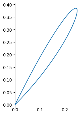
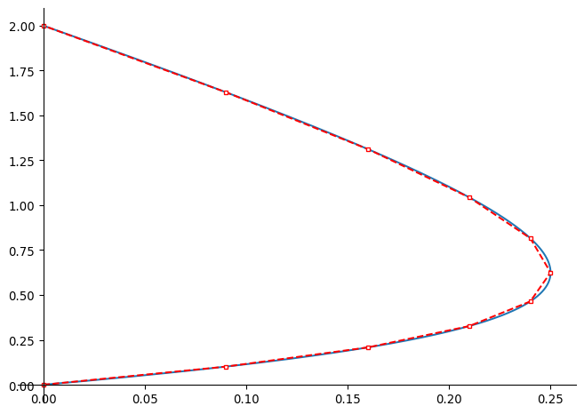
marker = {"color": "r", "marker": "s", "fillstyle":'full',"markerfacecolor":'white', "markersize":3, "linestyle":'--'}


t = sp.symbols('t')
f = t - t**2
g = t + t**3

# Evaluate functions at ten points 
numpoints = 10
tval = [i/numpoints for i in list(range(0,numpoints))] + [1]
fvals = [f.subs(t, t0 ) for t0 in tval]
gvals = [g.subs(t, t0 ) for t0 in tval]
marker["args"] = [fvals,gvals]

# Plot parameters
sp.plot_parametric(f,g, (t, 0, 1), markers = marker)

L = \int_a^b\sqrt{f'(t)^2 + g'(t)^2} dt

To make things convenient we will convert our operations into a function.

def _curvelength(f, g, var):
  """
  Inputs:
    f, g: x and y parametrizations
    var (tuple): (sp.symbol, lower lim, upper lim)

    var is a  the variable upon which to integrate.
  """
  t, a, b = var

  dx_dt = sp.diff(f, t)
  dy_dt = sp.diff(g, t)

  integ = (dx_dt**2 + dy_dt**2)
  integ = sp.sqrt(integ)
  _displayM("Integrating: ", integ)
  _displayM(f"over [{a}, {b}] w.r.t.", t)

  res = sp.integrate(integ, (t, a, b))
  print("gives:")

  return res

Example (circle/spiral)

t, r = sp.symbols('t r', positive = True)

f = r * sp.cos(t)
g = r * sp.sin(t)

_curvelength(f,g, (t, 0, 2 * sp.pi))

Integrating: \sqrt{r^{2} \sin^{2}{\left(t \right)} + r^{2} \cos^{2}{\left(t \right)}}

over [0, 2*pi] w.r.t. t

gives:

\displaystyle 2 \pi r

Example (astroid)

t = sp.symbols('t')

f = (sp.cos(t))**3
g = (sp.sin(t))**3


_curvelength(f,g, (t, 0, sp.pi/2))

Integrating: \sqrt{9 \sin^{4}{\left(t \right)} \cos^{2}{\left(t \right)} + 9 \sin^{2}{\left(t \right)} \cos^{4}{\left(t \right)}}

over [0, pi/2] w.r.t. t

gives:

\displaystyle \frac{3}{2}

Example (ellipse)

t, a, b = sp.symbols('t a b', positive=True)

f = a * sp.cos(t)
g = b * sp.sin(t)

_curvelength(f, g, (t, 0, sp.pi/2))

Integrating: \sqrt{a^{2} \sin^{2}{\left(t \right)} + b^{2} \cos^{2}{\left(t \right)}}

over [0, pi/2] w.r.t. t

gives:

\displaystyle \int\limits_{0}^{\frac{\pi}{2}} \sqrt{a^{2} \sin^{2}{\left(t \right)} + b^{2} \cos^{2}{\left(t \right)}}\, dt

This is a special integral called the complete elliptic integral of the second kind.

NoteElliptic Integrals

Elliptic integrals

Let’s take the parametrization again and look for a series solution.

dx_dt = sp.diff(f,t)
dy_dt = sp.diff(g,t)

ecc = sp.symbols('e')
# e = sp.sqrt(1 - (b/a)**2)



integrand = (dx_dt**2 + dy_dt**2)
integrand = integrand.subs({a: b/sp.sqrt(1-ecc**2),
                            sp.cos(t)**2: 1 - sp.sin(t**2)})
integrand

\displaystyle b^{2} \left(1 - \sin{\left(t^{2} \right)}\right) + \frac{b^{2} \sin^{2}{\left(t \right)}}{1 - e^{2}}

t, e = sp.symbols('t e')
f = sp.sqrt(1 - e**2 * sp.sin(t**2))
sp.series(f,t)

\displaystyle 1 - \frac{e^{2} t^{2}}{2} - \frac{e^{4} t^{4}}{8} + O\left(t^{6}\right)