Conic Sections

Some plotting routines. Click to expand

import numpy as np
import sympy as sp
import matplotlib.pyplot as plt
from sympy import plot_parametric, symbols
from IPython.display import display, Markdown
from functools import partial

## This is a 'partial function' so that we don't have to set figure size and aspect ratio every time.
splot = partial(plot_parametric, aspect_ratio = (1,1),size=(4,4),axis_center = (0,0))



def _plotter(x, y, create = False):
    if create: plt.figure(figsize=(6, 6))
    plt.plot(x, y)
    plt.gca().set_aspect('equal', adjustable='box')

    return

def _centeraxes():
    ax = plt.gca()
    # Move left y-axis and bottom x-axis to centre, passing through (0,0)

    ax.spines['left'].set_position('zero')
    ax.spines['bottom'].set_position('zero')

    # Eliminate upper and right axes
    ax.spines['right'].set_color('none')
    ax.spines['top'].set_color('none')

    # Show ticks in the left and lower axes only
    ax.xaxis.set_ticks_position('bottom')
    ax.yaxis.set_ticks_position('left')
    return

def _displayM(text, expr):
  """
  Display text and expression inline. 
  """
  display(Markdown('{} {}'.format(
            text,
            sp.latex(expr, mode='inline')
          ))
  )

In Cartesian

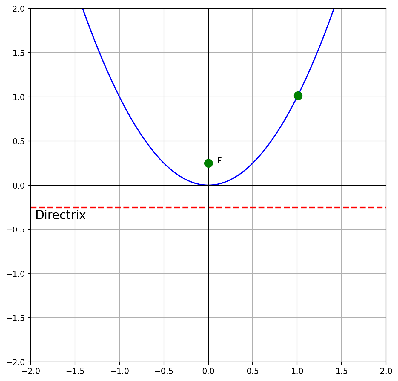
Parabola

%matplotlib inline

import numpy as np
import matplotlib.pyplot as plt

def conic(x, tp = 'parabola', p = {}):
  """
  x = values at which to compute
  tp = type of conic
  p = parameters
  """
  if tp == 'parabola': 
    y = p['a'] * (x - p['h'])**2 + p['k']
    focus = {'x': p['h'], 
              'y': p['k'] + 1/(4 * p['a'])}

  if tp == 'circle':
    circle_x = p['c_x'] + p['r'] * np.cos(x)
    circle_y = p['c_y'] + p['r'] * np.sin(x)

    return circle_x, circle_y


  return y, focus

## Generate parabola
x = np.linspace(-2, 2, 400)
params = {'a': 1, 'h': 0, 'k': 0}
y, focus = conic(x, 'parabola', p = params)

## Point of observation
ind = 300
pb_x, pb_y = np.abs(x[ind]), np.abs(y[ind])

# Plot
plt.figure(figsize=(8, 8))
plt.plot(x, y, label='$y = x^2$', color='blue')
plt.scatter(focus['x'], focus['y'], color='green', zorder=5, s=100)
plt.text(focus['x'] + 0.1, focus['y'], 'F')

plt.text(focus['x'] -1.95, -focus['y']-0.13, 'Directrix', fontsize= 15)

plt.scatter(pb_x, pb_y, color='green', zorder = 3, s = 100)

## Plot settings
plt.xlim(-2, 2)
plt.ylim(-2, 2)
plt.grid(True)
plt.axhline(-focus['y'], color='red', linewidth=2, ls = '--')
plt.axhline(0, color='black', linewidth=1)
plt.axvline(0, color='black', linewidth=1)

#__________________________________________

#==================================
### DO NOT DELETE (Uncomment to show circles)
#==================================

# ##=============== Circles 
# radius = np.sqrt((focus['x'] - pb_x)**2 + (focus['y'] - pb_y)**2)

# theta = np.linspace(0, 2 * np.pi, 400)

# ## Circle A
# params = {'c_x': focus['x'], 'c_y': focus['y'], 'r': radius}
# theta = np.linspace(0, 2 * np.pi, 400)
# circle_x, circle_y = conic(theta, 'circle', p = params)

# plt.plot(circle_x, circle_y, color='red')


# ## Circle B
# params = {'c_x': pb_x, 'c_y': -focus['y'], 'r': radius}
# circle_2x, circle_2y = conic(theta, 'circle', p = params)

# plt.plot(circle_2x, circle_2y, color='red')

# ## Lines
# plt.plot([pb_x, pb_x], [-focus['y'], pb_y], '--') #vertical dashed line
# plt.plot([0, pb_x], [focus['y'], pb_y], '--') #line from focus to parabola 

#__________________________


plt.show()

We can animate the circles to show how the distances from the focus to a point on the parabola, and a circle on directrix directly under the parabola are the same.

Parabola Animation

import numpy as np
import matplotlib.pyplot as plt
from matplotlib.animation import FuncAnimation
from IPython.display import HTML

# Use the notebook backend for interactive plots
%matplotlib notebook

# Set up the figure and axes
fig, ax = plt.subplots(figsize = [4,4])
xdata, ydata = [], []
circleA, = plt.plot([], [], 'r-')
circleB, = plt.plot([], [], 'r-')
point,   = plt.plot([], [], 'bo', zorder = 10, markersize = 10)

linev,   = plt.plot([], [], '--') #vertical dashed line
linef,   = plt.plot([], [], '--') #line from focus to parabola 

# Initialize the plot
def init():
    ax.set_xlim(0, 2 * np.pi)
    ax.set_ylim(-1, 1)

    #Create parabola, foci etc. 
    ## Generate parabola
    x = np.linspace(-2, 2, 400)
    params = {'a': 1, 'h': 0, 'k': 0}
    y, focus = conic(x, 'parabola', p = params)

    ## Plot Focus
    plt.plot(x, y, label='$y = x^2$', color='blue')
    plt.scatter(focus['x'], focus['y'], color='green', zorder=5, s=80)
    plt.text(focus['x'] + 0.1, focus['y'], 'F')

    ## Plot settings
    plt.xlim(-2, 2)
    plt.ylim(-2, 2)
    plt.grid(True)
    plt.axhline(-focus['y'], color='black', linewidth=1)
    plt.axvline(0, color='black', linewidth=1)
    return plt

# Update function for animation
def update(frames):


    ## Point of observation
    ind = frames 
    pb_x, pb_y = np.abs(x[ind]), np.abs(y[ind])
    point.set_data(pb_x, pb_y)
    

    ##=============== Circles 
    radius = np.sqrt((focus['x'] - pb_x)**2 + (focus['y'] - pb_y)**2)
    theta = np.linspace(0, 2 * np.pi, 400)

    ## Circle A
    params = {'c_x': focus['x'], 'c_y': focus['y'], 'r': radius}
    circle_x, circle_y = conic(theta, 'circle', p = params)
   
    circleA.set_data(circle_x, circle_y)

    ## Circle B
    params = {'c_x': pb_x, 'c_y': -focus['y'], 'r': radius}
    circle_2x, circle_2y = conic(theta, 'circle', p = params)

    circleB.set_data(circle_2x, circle_2y)

    ##============== Lines
    linev.set_data([pb_x, pb_x], [-focus['y'], pb_y])
    linef.set_data([0, pb_x], [focus['y'], pb_y])


    return 

# Create the animation
ani = FuncAnimation(
    fig, update, frames=list(range(200)),
    init_func=init, blit=True, interval=20
)

# Display the animation
HTML(ani.to_html5_video())

/tmp/ipykernel_23069/2707575446.py:50: MatplotlibDeprecationWarning:

Setting data with a non sequence type is deprecated since 3.7 and will be remove two minor releases later

Ellipse

Warning: The code below needs tweaking.

import numpy as np
import plotly.graph_objects as go
from plotly.subplots import make_subplots

# Function to generate ellipse points
def generate_ellipse(a, e, num_points=100):
    b = a * np.sqrt(1 - e**2)  # semi-minor axis
    theta = np.linspace(0, 2 * np.pi, num_points)
    x = a * np.cos(theta)
    y = b * np.sin(theta)
    return x, y

# Initial parameters
eccentricity = 0.5
semi_major_axis = 1
num_points = 100

# Create initial ellipse
x, y = generate_ellipse(semi_major_axis, eccentricity)

# Create the figure and add the initial ellipse
fig = make_subplots(rows=1, cols=1)
fig.add_trace(go.Scatter(x=x, y=y, mode='lines', name='Ellipse'))

# Set fixed axis limits
fig.update_layout(
    title=f'Ellipse with Semi-Major Axis = {semi_major_axis}, Eccentricity = {eccentricity:.2f}',
    xaxis_title='X',
    yaxis_title='Y',
    xaxis=dict(scaleanchor="y", range=[-2, 2]),
    yaxis=dict(constrain='domain', range=[-2, 2]),
    showlegend=False
)

# Create sliders for eccentricity and semi-major axis
fig.update_layout(
    sliders=[
        {
            'active': 0,
            'yanchor': 'top',
            'xanchor': 'left',
            'currentvalue': {
                'prefix': 'Eccentricity: ',
                'visible': True,
                'xanchor': 'right'
            },
            'pad': {'b': 10},
            'len': 0.9,
            'x': 0.1,
            'y': -0.1,
            'steps': [{
                'label': f'{i/100:.2f}',
                'method': 'update',
                'args': [{'x': [generate_ellipse(semi_major_axis, i/100)[0]], 
                                'y': [generate_ellipse(semi_major_axis, i/100)[1]]},
                          {'title': f'Ellipse with Semi-Major Axis = {semi_major_axis}, Eccentricity = {i/100:.2f}'}]
                } for i in range(0, 101, 10)]  # Eccentricity steps
        },
        {
            'active': 0,
            'yanchor': 'top',
            'xanchor': 'left',
            'currentvalue': {
                'prefix': 'Semi-Major Axis: ',
                'visible': True,
                'xanchor': 'right'
            },
            'pad': {'b': 10},
            'len': 0.9,
            'x': 0.1,
            'y': -0.3,
            'steps': [{
                'label': f'{i/10:.1f}',
                'method': 'update',
                'args': [{'x': [generate_ellipse(i/10, eccentricity)[0]], 
                             'y': [generate_ellipse(i/10, eccentricity)[1]]},
                          {'title': f'Ellipse with Semi-Major Axis = {i/10:.1f}, Eccentricity = {eccentricity:.2f}'}]
                } for i in range(1, 21)]  # Semi-major axis steps from 0.1 to 2.0
        }
    ]
)

# Show the figure
fig.show()

Conic Sections

In Cartesian

Parabola

Ellipse

Hyperbola

In Polar