Parametric Plots

Basic parametrizations

import numpy as np
import matplotlib.pyplot as plt

def plotter(x, y, create = False):
    if create: plt.figure(figsize=(6, 6))
    plt.plot(x, y)
    plt.gca().set_aspect('equal', adjustable='box')

    return

def centeraxes():
    ax = plt.gca()
    # Move left y-axis and bottom x-axis to centre, passing through (0,0)

    ax.spines['left'].set_position('zero')
    ax.spines['bottom'].set_position('zero')

    # Eliminate upper and right axes
    ax.spines['right'].set_color('none')
    ax.spines['top'].set_color('none')

    # Show ticks in the left and lower axes only
    ax.xaxis.set_ticks_position('bottom')
    ax.yaxis.set_ticks_position('left')
    return

Parabola

Circle and Ellipse

t = np.linspace(0, 2 * np.pi, 400)

x = np.cos(t)
y = np.sin(t)
plotter(x,y, create = True)

x = 2* np.cos(t)
y = np.sin(t)
plotter(x,y)
centeraxes()
plt.show()

Hyperpola

t = np.linspace(0.1, 10, 400)

x = t + 1/t
y = t - 1/t
plotter(x,y)
centeraxes()

plt.show()

Cycloid

t = np.linspace(0, 8*np.pi, 400)

a = 1

x = a * (t - np.sin(t))
y = a * (1 - np.cos(t))
plotter(x,y)
centeraxes()

plt.show()

Brachistochrone and Tautochrone

Miscellaneous

Drawing the Batman curve.

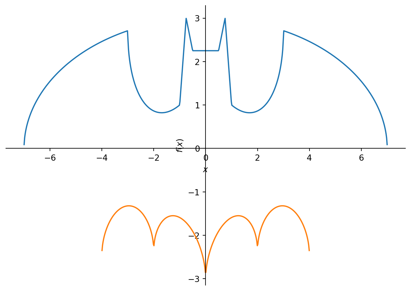
import numpy as np
import matplotlib.pyplot as plt
x = np.linspace(-6,6,1000)

def sf(x):
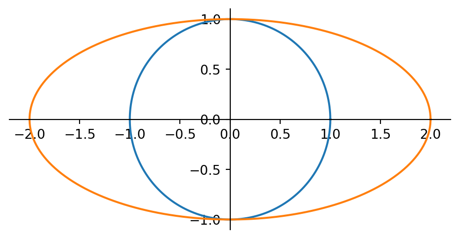
    return np.sqrt(1-x**2)                           # semicircle
def ef(x):
    return 3*sf(x/7)                             # ellipse
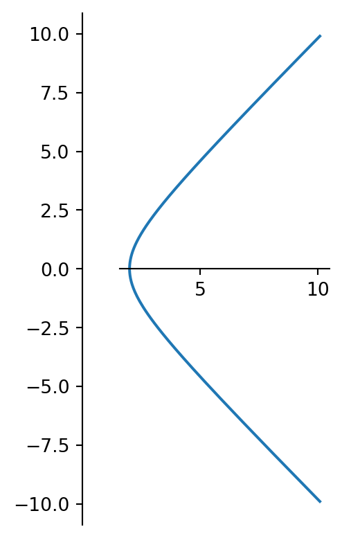
def sh(x):
    return 4.2 - .5*x -2.8*sf(.5*x -.5)          # shoulders
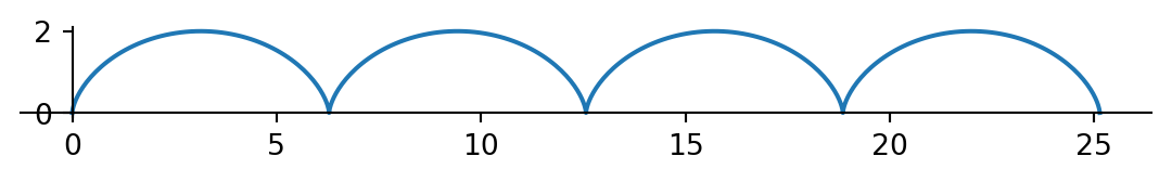
def bf(x):
    return sf(abs(2 - x) - 1) - x**2/11 + .5*x -3 # bottom

cl_x = [0,0.5,0.8,1]
cl_xn = [-x for x in cl_x]
cl_y = [1.7, 1.7, 2.6, 0.9]

def p(f,xmin,xmax, flipy = False):
    "symmetric plot across y-axis"
    
    x = np.linspace(xmin, xmax, 100)
    y = f(x)
    if flipy: 
        y = -y
    p1 = plt.plot(x, y)
    
    x = [-i for i in x]
    ax = plt.plot(x, y)
    
    return ax

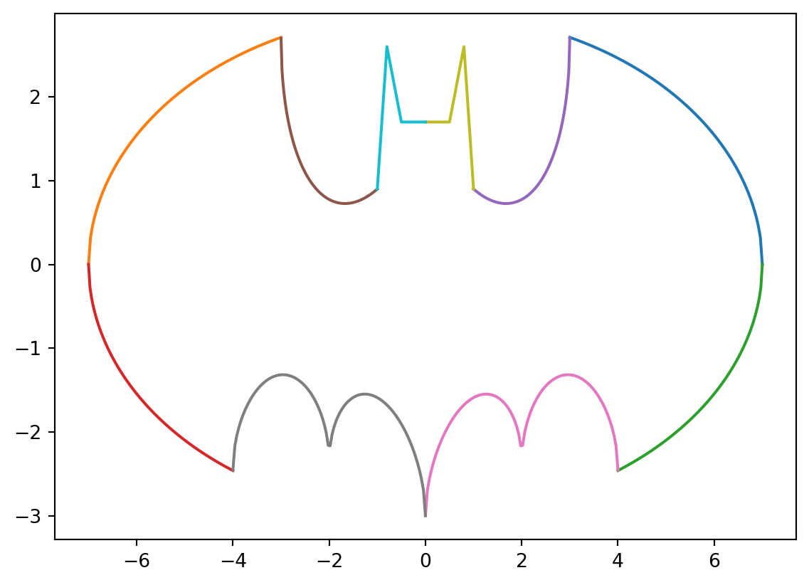
p(ef,3,7) 
p(ef,4,7, flipy = True) 
p(sh,1,3)
p(bf,0,4) 
plt.plot(cl_x, cl_y)
plt.plot(cl_xn, cl_y)
plt.show()

Below is a parametrized version of the plot.

import sympy as sm


x = sm.symbols('x', real=True)
h_ = sm.symbols('h_')

w = 3 * sm.sqrt(1 - (x / 7)**2)
l = ((x + 3) / 2 - sm.S(3) / 7 * sm.sqrt(10) * sm.sqrt(4 - (x + 1)**2) +
        sm.S(6) / 7 * sm.sqrt(10))
r = ((3 - x) / 2 - sm.S(3) / 7 * sm.sqrt(10) * sm.sqrt(4 - (x - 1)**2) +
        sm.S(6) / 7 * sm.sqrt(10))
h = (3*(sm.Abs(x - sm.S.Half) + sm.Abs(x + sm.S.Half) + 6) -
                11*(sm.Abs(x - sm.S(3)/4) + sm.Abs(x + sm.S(3)/4)))/2 
f = ((h - l) * sm.Heaviside(x + 1, 0) +
        (r - h) * sm.Heaviside(x - 1, 0) +
        (l - w) * sm.Heaviside(x + 3, 0) +
        (w - r) * sm.Heaviside(x - 3, 0) + 
        w)
g = (sm.S(1) / 2 * (sm.Abs(x / 2) + sm.sqrt(1 - (sm.Abs(sm.Abs(x) - 2) -
        1)**2) - sm.S(1) / 112 * (3 * sm.sqrt(33) - 7) * x**2 + 3 *
        sm.sqrt(1 - (sm.S(1) / 7 * x)**2) - 3) * ((x + 4) / sm.Abs(x + 4) -
        (x - 4) / sm.Abs(x - 4)) - 3 * sm.sqrt(1 - (x / 7)**2))
sm.plot(f, g)

<lambdifygenerated-3>:2: RuntimeWarning: invalid value encountered in sqrt
  return -3*sqrt(1 - 1/49*x**2) + (-(x - 4)/abs(x - 4) + (x + 4)/abs(x + 4))*(-1/2*x**2*(-1/16 + (3/112)*sqrt(33)) + (3/2)*sqrt(1 - 1/49*x**2) + (1/2)*sqrt(1 - (abs(abs(x) - 2) - 1)**2) + (1/4)*abs(x) - 3/2)

The bottom wings are missing. Most likely some part of the equation is missing. You can experiment with the equations if you want.

Taken from Math World