Vectors and Geometry of Space

Contour plots

import matplotlib as mpl
from mpl_toolkits.mplot3d import Axes3D
import numpy as np
import matplotlib.pyplot as plt

# mpl.rcParams['legend.fontsize'] = 10

fig = plt.figure()
ax = fig.add_subplot(projection = '3d')

theta = np.linspace(0, 2 * np.pi, 100)
z = 0
r = 1
x = r * np.sin(theta)
y = r * np.cos(theta)
ax.plot(x, y, z)

## We can shift the same plot by choosing different values of z.
# z = 3
# ax.plot(x, y, z)

## for z in np.linspace(0, 1, 100):
##   ax.plot(x, y, z)

plt.show()

But what if we link r and z?

# mpl.rcParams['legend.fontsize'] = 10

fig = plt.figure()
ax = fig.add_subplot(projection = '3d')

theta = np.linspace(0, 2 * np.pi, 100)
z = 0
r = 1
x = r * np.sin(theta)
y = r * np.cos(theta)
ax.plot(x, y, z)

## We can shift the same plot by choosing different values of z.
# z = 3
# ax.plot(x, y, z)

## for z in np.linspace(0, 1, 100):
##   ax.plot(x, y, z)

plt.show()

Region plot (inequalities)

# from itertools import product

# def cartesian_product(*arrays):
#     la = len(arrays)
#     dtype = np.result_type(*arrays)
#     arr = np.empty([len(a) for a in arrays] + [la], dtype=dtype)
#     for i, a in enumerate(np.ix_(*arrays)):
#         arr[...,i] = a
#     return arr.reshape(-1, la)


# fig = plt.figure()
# ax = fig.add_subplot(projection='3d')


# xd = np.linspace(0,1,100)
# yd = np.linspace(0,1,100)
# zd = np.linspace(0,1,100)
# products =   cartesian_product(xd, yd, zd)


# for x, y, z in products:
    
#     ax.scatter(x, y, z)



# ax.set_xlabel('X Label')
# ax.set_ylabel('Y Label')
# ax.set_zlabel('Z Label')

# plt.show()

Vectors in sympy

from sympy.vector import CoordSys3D
N = CoordSys3D('N')

v = 2*N.i + N.j #Defines a vector

from sympy.vector import Vector
Vector.zero
type(Vector.zero)
N.i + Vector.zero
Vector.zero == 2*Vector.zero

True

Dot(&) and Cross product(^):

v1 = 2*N.i + 3*N.j - N.k
v2 = N.i - 4*N.j + N.k
v1.dot(v2)
v1.cross(v2)
v2.cross(v1)


v1 & v2
v1 ^ v2

\(\displaystyle - \mathbf{\hat{i}_{N}} + \left(-3\right)\mathbf{\hat{j}_{N}} + \left(-11\right)\mathbf{\hat{k}_{N}}\)

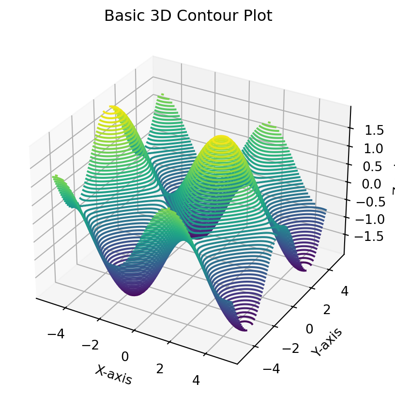
%matplotlib inline

import matplotlib.pyplot as plt
import numpy as np
from mpl_toolkits.mplot3d import Axes3D

# Creating data
x = np.linspace(-5, 5, 100)
y = np.linspace(-5, 5, 100)
X, Y = np.meshgrid(x, y)
Z = np.sin(X) + np.cos(Y)

# Creating a 3D plot
fig = plt.figure()
ax = fig.add_subplot(111, projection='3d')

# Plotting the 3D contour
ax.contour3D(X, Y, Z, 50, cmap='viridis')

# Customizing the plot
ax.set_xlabel('X-axis')
ax.set_ylabel('Y-axis')
ax.set_zlabel('Z-axis')
ax.set_title('Basic 3D Contour Plot')

# Displaying the plot
plt.show()

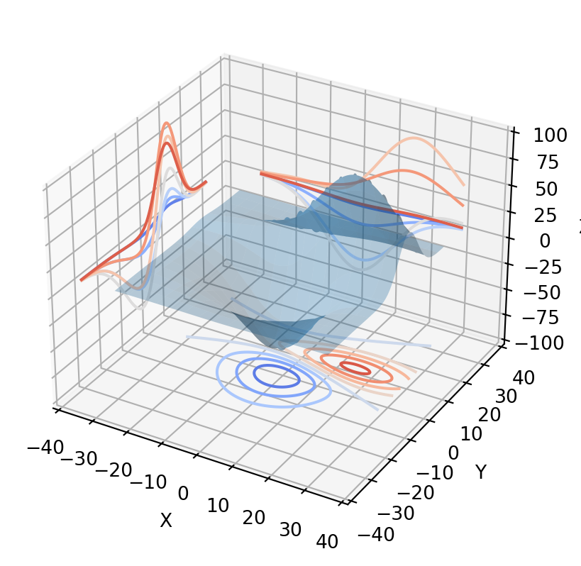
from mpl_toolkits.mplot3d import axes3d
import matplotlib.pyplot as plt
from matplotlib import cm

fig = plt.figure()
ax = fig.add_subplot(projection = '3d')

X, Y, Z = axes3d.get_test_data(0.05)
ax.plot_surface(X, Y, Z, rstride=8, cstride=8, alpha=0.3)
cset = ax.contour(X, Y, Z, zdir='z', offset=-100, cmap=cm.coolwarm)
cset = ax.contour(X, Y, Z, zdir='x', offset=-40, cmap=cm.coolwarm)
cset = ax.contour(X, Y, Z, zdir='y', offset=40, cmap=cm.coolwarm)

ax.set_xlabel('X')
ax.set_xlim(-40, 40)
ax.set_ylabel('Y')
ax.set_ylim(-40, 40)
ax.set_zlabel('Z')
ax.set_zlim(-100, 100)

plt.show()

import plotly.graph_objects as go
import numpy as np
np.random.seed(1)

N = 70

fig = go.Figure(data=[go.Mesh3d(x=(70*np.random.randn(N)),
                   y=(55*np.random.randn(N)),
                   z=(40*np.random.randn(N)),
                   opacity=0.5,
                   color='rgba(244,22,100,0.6)'
                  )])

fig.update_layout(
    scene = dict(
        xaxis = dict(nticks=4, range=[-100,100],),
                     yaxis = dict(nticks=4, range=[-50,100],),
                     zaxis = dict(nticks=4, range=[-100,100],),),
    width=700,
    margin=dict(r=20, l=10, b=10, t=10))

fig.show()