import pandas as pd
import sympy as sp

marker = {"color": "r", "marker": "s", "fillstyle":'full',"markerfacecolor":'white', "markersize":10, "linestyle":'--'}Limits and Continuity
Averages
x = sp.symbols('x')

y = 4.9 * x**2

evalat = [1,2,3,4,5]
result = [y.subs(x, i).evalf(3) for i in evalat]

xypairs = list(zip(evalat, result))

pd.DataFrame(xypairs, columns = ['x', 'y'])| x | y | |
|---|---|---|
| 0 | 1 | 4.90 |
| 1 | 2 | 19.6 |
| 2 | 3 | 44.1 |
| 3 | 4 | 78.4 |
| 4 | 5 | 123. |
x = sp.symbols('x')
func = 4.9 * x**2

evalat = [1, 3, 7]
y = [func.subs(x, val) for val in evalat]

marker['args'] = [evalat, y] #See presets at top

sp.plot(func, (x,-1,7),
markers = marker,
annotations=[{'xy': (3, 120), 'text': "Secant", 'fontsize':15}]
)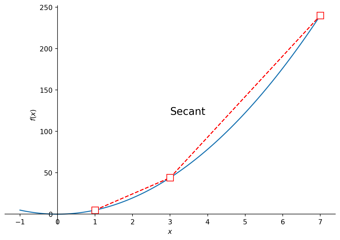
<sympy.plotting.backends.matplotlibbackend.matplotlib.MatplotlibBackend at 0x14a56deef0a0>We can also evaluate this numerically:
Limits
Of rational functions
# Limits of rational functions

x = sp.symbols('x')
p = x**3 + 4*x**2 - 3
q = x**2 + 5

rp = p/q

evalat = -1
result = sp.limit(rp, x, evalat)

# sp.plot(rp, (x, -2,0))
marker['args'] = [evalat, result]

sp.plot(rp, (x, -2,0), markers = marker)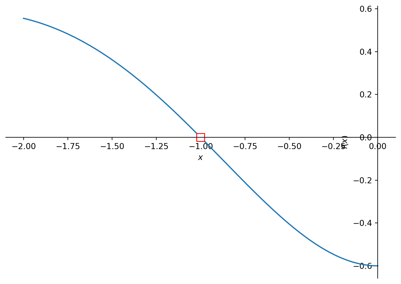
<sympy.plotting.backends.matplotlibbackend.matplotlib.MatplotlibBackend at 0x14a52e4ef8b0>Example - Limit with denominator 0
import sympy as sp
x = sp.symbols('x')

f = (sp.sqrt(x**2 + 100) - 10)/ x**2

sp.plot(f, (x, -1 , 1))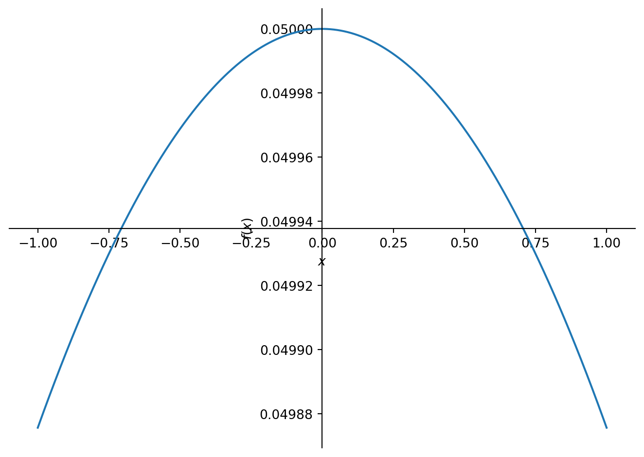
<sympy.plotting.backends.matplotlibbackend.matplotlib.MatplotlibBackend at 0x14a53ae4f4c0>Sandwich theorem
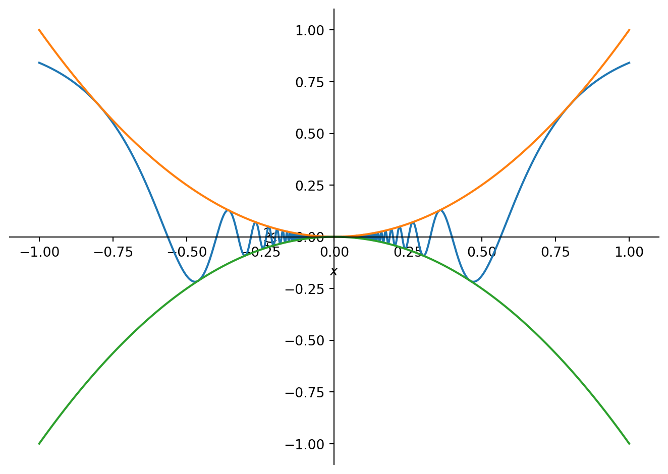
import sympy as sp
x = sp.symbols('x')

xi, xf = -1,1

f = x**2 * sp.sin(1/x**2)
upper = x**2
lower = -x**2

sp.plot(f, (x, xi , xf))

sp.plot((f, (x, xi , xf)),
        (upper, (x,xi, xf)),
        (lower, (x, xi, xf))
)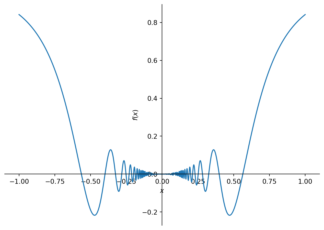
<sympy.plotting.backends.matplotlibbackend.matplotlib.MatplotlibBackend at 0x14a52ef842e0>One-sided limits
Limits (Rigorous definition)
Limits involving infinity
Oblique asymptotes
x = sp.symbols('x')
f = (x**3 - 8)/(x-4)

sp.limit(f,x, 0)

sp.plot(f, (x,3.99,4.01))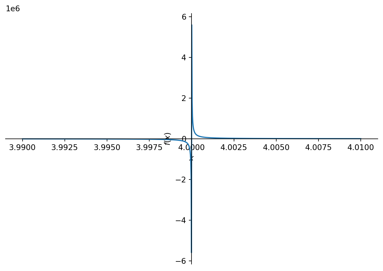
<sympy.plotting.backends.matplotlibbackend.matplotlib.MatplotlibBackend at 0x14a52ee63bb0>