Functions

Read: Chapter 1

Terminology

Following is a list of terms that you should know the meaning of.

• What are functions?
  • Vertical line test for a function.
  • Piece-wise defined functions
• Independent vs. dependent variables.
• Domain vs. range.
  • Closed vs. open intervals

Functions: Some properties

• Increasing vs. decreasing
• Even vs. odd
• Linear vs. non-linear

Plotting functions

import numpy as np
import matplotlib.pyplot as plt

def centeraxes():
  """Centers axes in the middle"""
  ax = plt.gca()
  ax.spines['top'].set_color('none')
  ax.spines['left'].set_position('zero')
  ax.spines['right'].set_color('none')
  ax.spines['bottom'].set_position('zero')
  return ax

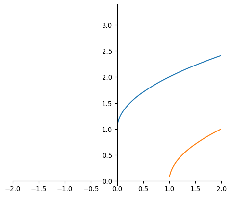
We can plot a single function as follows:

domain = np.linspace(-5,5, 1000)
func = np.sqrt(domain) + 1
func2 = np.sqrt(domain-1)
# plt.plot(domain, func)
# plt.plot(domain, func2)
plt.plot(domain, func)
plt.plot(domain, func2)
plt.xlim([-2,2])
plt.gca().set_aspect('equal')

centeraxes()

plt.show()

/tmp/ipykernel_85732/4150367370.py:2: RuntimeWarning:

invalid value encountered in sqrt

/tmp/ipykernel_85732/4150367370.py:3: RuntimeWarning:

invalid value encountered in sqrt

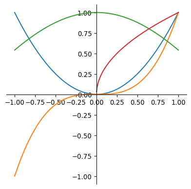
But we can also plot multiple functions, although this is not necessarily the neatest way, Matplotlib changes colors by default (but we can control it too):

import numpy as np
import matplotlib.pyplot as plt

domain = np.linspace(-1,1, 1000)
func = domain**2
func2 = domain**3
func3 = np.cos(domain)
func4 = np.sqrt(domain)

plt.plot(domain, func)
plt.plot(domain, func2)
plt.plot(domain, func3)
plt.plot(domain, func4)
plt.gca().set_aspect('equal')

centeraxes()

plt.show()

/tmp/ipykernel_85732/3654791602.py:8: RuntimeWarning:

invalid value encountered in sqrt

import sympy as sp

x = sp.symbols('x')
y = x**2 + x
y2 = x**3

sp.plot(y, y2, (x, 0, 2) )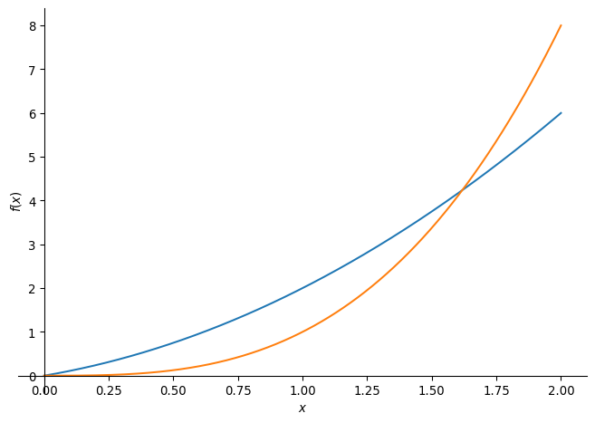

Some special functions

Linear functions

Absolute value function/Modulus

Power functions

Polynomials

Rational functions

Algebraic functions

Trigonometric functions

import sympy as sp

# Define the variable
x = sp.Symbol('x')

func1 = sp.cos(x)
func2 = sp.sec(x)

func3 = sp.sin(x)
func4 = sp.csc(x)

func5 = sp.tan(x)
func6 = sp.cot(x)
# Define the piecewise function

# Display the piecewise function
sp.plot(func2, func3, (x,-4*sp.pi,4*sp.pi), ylim = (-2,2))

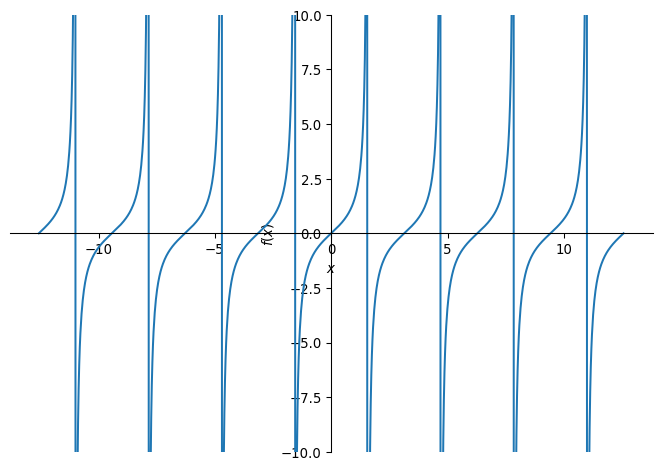
sp.plot(func5, (x,-4*sp.pi,4*sp.pi), ylim = (-10,10))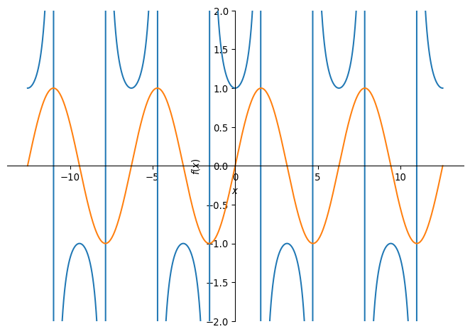

Inverse Trigonometric

import sympy as sp

# Define the variable
x = sp.Symbol('x')

func1 = sp.acos(x)
func2 = sp.asec(x)

func3 = sp.asin(x)
func4 = sp.acsc(x)

func5 = sp.atan(x)
func6 = sp.acot(x)
# Define the piecewise function

# Display the piecewise function
sp.plot(func2, func3, (x,-4*sp.pi,4*sp.pi), ylim = (-2,2))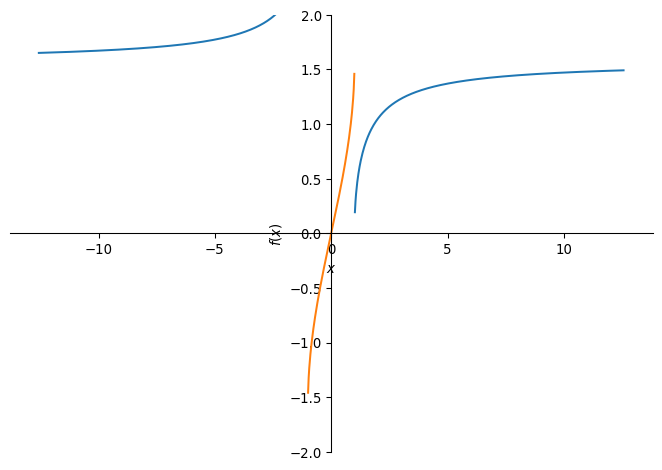

Exponential functions

Logarithmic functions

Transcendental functions

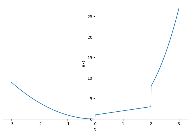
Piecewise

import sympy as sp

# Define the variable
x = sp.Symbol('x')

# Define the piecewise function
piecewise_func = sp.Piecewise(
    (x**2, x < 0),        # x^2 when x < 0
    (x + 1, (x >= 0) & (x <= 2)),  # x + 1 when 0 <= x <= 2
    (x**3, x > 2)         # x^3 when x > 2
)

# Display the piecewise function
sp.plot(piecewise_func, (x,-3,3))